15.5 第一个模型:线性回归
普通最小二乘法线性回归在众多回归模型家族中是最简单的一个。用于计算它的函数是名字非常简约的lm(即线性模型linear model的缩写)。它接受我们刚刚讨论过的公式类型,以及一个包含变量模型的数据框。来看一看gonorrhoea数据集。为简单起见,我们将忽略交互:
model1 <- lm(Rate ~ Year + Age.Group + Ethnicity + Gender, gonorrhoea)
如果我们打印出此模型变量,它将列出了每个输入变量的系数(αi的值) 。如果仔细观察你会发现,对于我们放进模型的两个类别变量(age group和ethnicity),其中一个没有系数。例如,看不到0 to 4的年龄组,而American Indians & Alaskan Natives民族也不翼而飞。
这些“缺失”的类别被包含在截距中。在下面的输出中,截距中的5540人为0~4岁的美洲印第安人和阿拉斯加土著女性中每10万人在第0年感染淋病的数量。为了预测2013年的总感染率,加上2013乘以Year的系数-2.77。为了预测在25到29岁同种族的感染率,加上该年龄组的系数291:
model1#### Call:## lm(formula = Rate ~ Year + Age.Group + Ethnicity + Gender, data = gonorrhoea)#### Coefficients:#### (Intercept) Year## 5540.496 -2.770## Age.Group5 to 9 Age.Group10 to 14## -0.614 15.268## Age.Group15 to 19 Age.Group20 to 24## 415.698 546.820## Age.Group25 to 29 Age.Group30 to 34## 291.098 155.872## Age.Group35 to 39 Age.Group40 to 44## 84.612 49.506## Age.Group45 to 54 Age.Group55 to 64## 27.364 8.684## Age.Group65 or more EthnicityAsians & Pacific Islanders## 1.178 -82.923## EthnicityHispanics EthnicityNon-Hispanic Blacks## -49.000 376.204## EthnicityNon-Hispanic Whites GenderMale## -68.263 -17.892
“0- to 4-year-old female American Indians and Alaskan Natives”(0到4岁美洲印第安人和阿拉斯加土著女性)组被选中,是因为它包含了每个因子变量的第一级。我们可以通过遍历数据集和调用levels来查看这些因子水平:
lapply(Filter(is.factor, gonorrhoea), levels)## $Age.Group## [1] "0 to 4" "5 to 9" "10 to 14" "15 to 19" "20 to 24"## [6] "25 to 29" "30 to 34" "35 to 39" "40 to 44" "45 to 54"## [11] "55 to 64" "65 or more"#### $Ethnicity## [1] "American Indians & Alaskan Natives"## [2] "Asians & Pacific Islanders"## [3] "Hispanics"## [4] "Non-Hispanic Blacks"## [5] "Non-Hispanic Whites"#### $Gender## [1] "Female" "Male"
除了知道每个输入变量的影响大小之外,我们通常还想知道哪些变量是最重要的。summary函数被重载了,它可与lm一起工作来做到这一点。summary输出中最令人兴奋的就是其系数表。Estimate列显示了我们已看到过的系数,以及第四列Pr(>|t|)显示了p值。第五列给出了一个星级评定:所在p值小于0.05的变量得到一星,小于0.01为二星级,以此类推。这使得它便于快速查看哪些变量有显著效果:
summary(model1)## Call:## lm(formula = Rate ~ Year + Age.Group + Ethnicity + Gender, data = gonorrhoea)#### Residuals:## Min 1Q Median 3Q Max## -376.7 -130.6 37.1 90.6 1467.1#### Coefficients:## Estimate Std. Error t value Pr(>|t## (Intercept) 5540.496 14866.406 0.37 0.709## Year -2.770 7.400 -0.37 0.708## Age.Group5 to 9 -0.614 51.268 -0.01 0.990## Age.Group10 to 14 15.268 51.268 0.30 0.766## Age.Group15 to 19 415.698 51.268 8.11 3.0e-1## Age.Group20 to 24 546.820 51.268 10.67 < 2e-1## Age.Group25 to 29 291.098 51.268 5.68 2.2e-0## Age.Group30 to 34 155.872 51.268 3.04 0.002## Age.Group35 to 39 84.612 51.268 1.65 0.099## Age.Group40 to 44 49.506 51.268 0.97 0.334## Age.Group45 to 54 27.364 51.268 0.53 0.593## Age.Group55 to 64 8.684 51.268 0.17 0.865## Age.Group65 or more 1.178 51.268 0.02 0.981## EthnicityAsians & Pacific Islanders -82.922 33.093 -2.51 0.012## EthnicityHispanics -49.000 33.093 -1.48 0.139## EthnicityNon-Hispanic Blacks 376.204 33.093 11.37 < 2e-1## EthnicityNon-Hispanic Whites -68.263 33.093 -2.06 0.039## GenderMale -17.892 20.930 -0.85 0.393#### (Intercept)## Year## Age.Group5 to 9## Age.Group10 to 14## Age.Group15 to 19 ***## Age.Group20 to 24 ***## Age.Group25 to 29 ***## Age.Group30 to 34 **## Age.Group35 to 39 .## Age.Group40 to 44## Age.Group45 to 54## Age.Group55 to 64## Age.Group65 or more## EthnicityAsians & Pacific Islanders *## EthnicityHispanics## EthnicityNon-Hispanic Blacks ***## EthnicityNon-Hispanic Whites *## GenderMale## ---## Signif. codes: 0 '***' 0.001 '**' 0.01 '*' 0.05 '.' 0.1 ' ' 1#### Residual standard error: 256 on 582 degrees of freedom## Multiple R-squared: 0.491, Adjusted R-squared: 0.476## F-statistic: 33.1 on 17 and 582 DF, p-value: <2e-16
15.5.1 比较和更新模型
通常,我们不会满足于所得到的第一个模型,而是想找到“最佳”模型或一些能提供洞见的模型。
本节展示了一些用于测量模型质量的指标,如p值和对数似然测量。通过使用这些指标来比较模型,你可以不断地自动更新模型,直到找到一个“最佳”模型为止。
不幸的是,像这样的模型自动更新(逐步回归)对于选择模型来说不是一个好的方法,而且当你增加了输入变量的数量,它会变得更糟。
更好的模型选择方法,如模型培训或模型平均,本书不作讨论。网站CrossValidated statistics Q&A site(http://bit.ly/1a5q6IQ)列举了一些比较好方法。
提示
试图找到“最佳”模型本身就是错的。好的模型即能对你的问题有所启发,而这样的模型可能有多个。
为了明智地给我们的数据选择一个模型,我们需要对影响淋病感染率的因素有所了解。淋病主要通过性传播(有一些是在母亲分娩的过程中传染给了婴儿),所以它最主要的驱动因素与性文化有关:如有多少个性伙伴,进行过多少次没有保护措施的性行为。
对于Year的p值是0.71,这意味着它的影响还谈不上显著。在如此短的时间内(五年的数据),如果性文化上有任何变化能对感染率产生重要的影响,我会感到很惊讶,所以看看如果删除它会发生什么。
无须重新指定模型,我们可以使用update函数修改它。它接受一个模型和公式为输入参数。我们只更新公式的右边,左边保持不变。在下例中,.的意思是:此项已在公式中,而减号-的意思是:删除此下一项:
model2 <- update(model1, ~ . - Year)summary(model2)#### Call:## lm(formula = Rate ~ Age.Group + Ethnicity + Gender, data = gonorrhoea)#### Residuals:## Min 1Q Median 3Q Max## -377.6 -128.4 34.6 92.2 1472.6#### Coefficients:## Estimate Std. Error t value Pr(>|t)## (Intercept) -25.10 43.116 -0.58 0.5606## Age.Group5 to 9 -0.614 51.230 -0.01 0.9904## Age.Group10 to 14 15.268 51.230 0.30 0.7658## Age.Group15 to 19 415.698 51.230 8.11 2.9e-15## Age.Group20 to 24 546.820 51.230 10.67 < 2e-16## Age.Group25 to 29 291.098 51.230 5.68 2.1e-08## Age.Group30 to 34 155.872 51.230 3.04 0.0025## Age.Group35 to 39 84.612 51.230 1.65 0.0992## Age.Group40 to 44 49.506 51.230 0.97 0.3343## Age.Group45 to 54 27.364 51.230 0.53 0.5934## Age.Group55 to 64 8.684 51.230 0.17 0.8655## Age.Group65 or more 1.178 51.230 0.02 0.9817## EthnicityAsians & Pacific Islanders -82.923 33.069 -2.51 0.0124## EthnicityHispanics -49.000 33.069 -1.48 0.1389## EthnicityNon-Hispanic Blacks 376.204 33.069 11.38 < 2e-16## EthnicityNon-Hispanic Whites -68.263 33.069 -2.06 0.0394## GenderMale -17.892 20.915 -0.86 0.3926#### (Intercept)## Age.Group5 to 9## Age.Group10 to 14## Age.Group15 to 19 ***## Age.Group20 to 24 ***## Age.Group25 to 29 ***## Age.Group30 to 34 **## Age.Group35 to 39 .## Age.Group40 to 44## Age.Group45 to 54## Age.Group55 to 64## Age.Group65 or more## EthnicityAsians & Pacific Islanders *## EthnicityHispanics## EthnicityNon-Hispanic Blacks ***## EthnicityNon-Hispanic Whites *## GenderMale## ---## Signif. codes: 0 '***' 0.001 '**' 0.01 '*' 0.05 '.' 0.1 ' ' 1#### Residual standard error: 256 on 583 degrees of freedom## Multiple R-squared: 0.491, Adjusted R-squared: 0.477## F-statistic: 35.2 on 16 and 583 DF, p-value: <2e-16
anova函数能计算模型的方差分析表(ANalysis Of VAriance),让你看到简化模型与全面的模型相比是否有显著区别:
anova(model1, model2)## Analysis of Variance Table#### Model 1: Rate ~ Year + Age.Group + Ethnicity + Gender## Model 2: Rate ~ Age.Group + Ethnicity + Gender## Res.Df RSS Df Sum of Sq F Pr(>F)## 1 582 38243062## 2 583 38252272 -1 -9210 0.14 0.71
右边列中的p值是0.71,所以删除year一项并没有显著影响拟合此数据的模型。
赤池(Akaike)和贝叶斯( Bayesian)信息准则提供了另外两种比较模型的方法,即AIC和BIC函数。它们利用了对数似然值,它们能告诉你用这个模型来拟合数据会有多好,而且会根据模型的项数多少决定如何作出惩罚(所以简单的模型比复杂的更好)。大致上较小的数字对应于“更好”的模型:
AIC(model1, model2)## df AIC## model1 19 8378## model2 18 8376BIC(model1, model2)## df BIC## model1 19 8462## model2 18 8456
通过创建一个“不靠谱”的模型,你能更好地了解这些函数的影响。让我们删除age group,它最能影响淋病感染率的预测(理应如此,儿童和老年人比青壮年的性行为要少得多):
silly_model <- update(model1, ~ . - Age.Group)anova(model1, silly_model)## Analysis of Variance Table#### Model 1: Rate ~ Year + Age.Group + Ethnicity + Gender## Model 2: Rate ~ Year + Ethnicity + Gender## Res.Df RSS Df Sum of Sq F Pr(>F)## 1 582 38243062## 2 593 57212506 -11 -1.9e+07 26.2 <2e-16 ***## ---## Signif. codes: 0 '***' 0.001 '**' 0.01 '*' 0.05 '.' 0.1 ' ' 1AIC(model1, silly_model)## df AIC## model1 19 8378## silly_model 8 8598BIC(model1, silly_model)## df BIC## model1 19 8462## silly_model 8 8633
在这个“不靠谱”模型中,anova指出模型间的显著差异,而且AIC和BIC都涨了不少。
继续寻找我们的“靠谱”模型,注意到性别是不显著的(p=0.39)。如果你做了练习14-3 (你已经完成了,是吧?),那么这对你来说可能是有趣的,因为从绘图中看起来妇女的感染率会更高。保留这种想法,直到你做完本章结尾的练习再看看。现在,让我们信任此p值,并从模型中删除性别gender项:
model3 <- update(model2, ~ . - Gender)summary(model3)#### Call:## lm(formula = Rate ~ Age.Group + Ethnicity, data = gonorrhoea)#### Residuals:## Min 1Q Median 3Q Max## -380.1 -136.1 35.8 87.4 1481.5#### Coefficients:## Estimate Std. Error t value Pr(>|t|)## (Intercept) -34.050 41.820 -0.81 0.4159## Age.Group5 to 9 -0.614 51.218 -0.01 0.9904## Age.Group10 to 14 15.268 51.218 0.30 0.7657## Age.Group15 to 19 415.698 51.218 8.12 2.9e-15## Age.Group20 to 24 546.820 51.218 10.68 < 2e-16## Age.Group25 to 29 291.098 51.218 5.68 2.1e-08## Age.Group30 to 34 155.872 51.218 3.04 0.0024## Age.Group35 to 39 84.612 51.218 1.65 0.0991## Age.Group40 to 44 49.506 51.218 0.97 0.3342## Age.Group45 to 54 27.364 51.218 0.53 0.5934## Age.Group55 to 64 8.684 51.218 0.17 0.8654## Age.Group65 or more 1.178 51.218 0.02 0.9817## EthnicityAsians & Pacific Islanders -82.923 33.061 -2.51 0.0124## EthnicityHispanics -49.000 33.061 -1.48 0.1389## EthnicityNon-Hispanic Blacks 376.204 33.061 11.38 < 2e-16## EthnicityNon-Hispanic Whites -68.263 33.061 -2.06 0.0394#### (Intercept)## Age.Group5 to 9## Age.Group10 to 14## Age.Group15 to 19 ***## Age.Group20 to 24 ***## Age.Group25 to 29 ***## Age.Group30 to 34 **## Age.Group35 to 39 .## Age.Group40 to 44## Age.Group45 to 54## Age.Group55 to 64## Age.Group65 or more## EthnicityAsians & Pacific Islanders *## EthnicityHispanics## EthnicityNon-Hispanic Blacks ***## EthnicityNon-Hispanic Whites *## ---## Signif. codes: 0 '***' 0.001 '**' 0.01 '*' 0.05 '.' 0.1 ' ' 1#### Residual standard error: 256 on 584 degrees of freedom## Multiple R-squared: 0.491, Adjusted R-squared: 0.477## F-statistic: 37.5 on 15 and 584 DF, p-value: <2e-16
最后,截距项看起来是不显著的。这是因为默认组为0~4岁的美洲印第安人和阿拉斯加土著,他们没有太多的淋病患者。
可以使用relevel函数设置不同的默认值。作为一个在30~34岁的非西班牙裔白人2,我将有意把这个设定为默认值。在下例中,请注意,我们可以使用update函数来更新数据框及公式:
2请提醒我在第二版时更改此项!
g2 <- within(gonorrhoea,{Age.Group <- relevel(Age.Group, "30 to 34")Ethnicity <- relevel(Ethnicity, "Non-Hispanic Whites")})model4 <- update(model3, data = g2)summary(model4)#### Call:## lm(formula = Rate ~ Age.Group + Ethnicity, data = g2)#### Residuals:## Min 1Q Median 3Q Max## -380.1 -136.1 35.8 87.4 1481.5#### Coefficients:## Estimate Std. Error t value## (Intercept) 53.6 41.8 1.28## Age.Group0 to 4 -155.9 51.2 -3.04## Age.Group5 to 9 -156.5 51.2 -3.06## Age.Group10 to 14 -140.6 51.2 -2.75## Age.Group15 to 19 259.8 51.2 5.07## Age.Group20 to 24 390.9 51.2 7.63## Age.Group25 to 29 135.2 51.2 2.64## Age.Group35 to 39 -71.3 51.2 -1.39## Age.Group40 to 44 -106.4 51.2 -2.08## Age.Group45 to 54 -128.5 51.2 -2.51## Age.Group55 to 64 -147.2 51.2 -2.87## Age.Group65 or more -154.7 51.2 -3.02## EthnicityAmerican Indians & Alaskan Natives 68.3 33.1 2.06## EthnicityAsians & Pacific Islanders -14.7 33.1 -0.44## EthnicityHispanics 19.3 33.1 0.58## EthnicityNon-Hispanic Blacks 444.5 33.1 13.44## Pr(>|t|)## (Intercept) 0.2008## Age.Group0 to 4 0.0024 **## Age.Group5 to 9 0.0024 **## Age.Group10 to 14 0.0062 **## Age.Group15 to 19 5.3e-07 ***## Age.Group20 to 24 9.4e-14 ***## Age.Group25 to 29 0.0085 **## Age.Group35 to 39 0.1647## Age.Group40 to 44 0.0383 *## Age.Group45 to 54 0.0124 *## Age.Group55 to 64 0.0042 **## Age.Group65 or more 0.0026 **## EthnicityAmerican Indians & Alaskan Natives 0.0394 *## EthnicityAsians & Pacific Islanders 0.6576## EthnicityHispanics 0.5603## EthnicityNon-Hispanic Blacks < 2e-16 ***## ---## Signif. codes: 0 '***' 0.001 '**' 0.01 '*' 0.05 '.' 0.1 ' ' 1#### Residual standard error: 256 on 584 degrees of freedom## Multiple R-squared: 0.491, Adjusted R-squared: 0.477## F-statistic: 37.5 on 15 and 584 DF, p-value: <2e-16
因为现在参考点不同了,所以系数和p值也改变了,但还是有很多的星号出现在右侧的摘要输出,所以我们得知年龄和种族对感染率有影响。
15.5.2 绘图和模型检查
lm模型有一个plot方法允许以6种不同的方式检查拟合度的好坏。在其最简单的形式中,你可以直接调用plot(the_model),它会逐张把图形绘制出来。稍好的方法是使用layout函数来一并查看所有的图,如图15-2所示 :
plot_numbers <- 1:6layout(matrix(plot_numbers, ncol = 2, byrow = TRUE))plot(model4, plot_numbers)
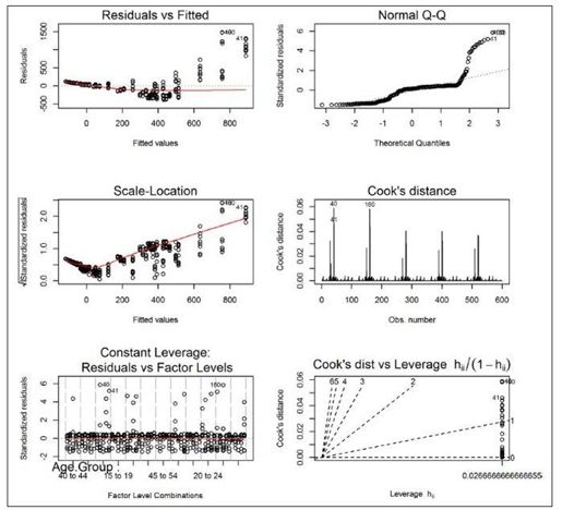
图15-2:诊断图的线性模型
在最上面,有一些值过高(注意在“Residuals vs Fitted”绘图中右侧出现的大的正残差,那些点远高于“Normal Q-Q”绘图中的线,以及出现在“Cook's distance”绘图中的峰值)。特别是第 40、41和160行已被挑选出来作为异常值:
gonorrhoea[c(40, 41, 160), ]## Year Age.Group Ethnicity Gender Rate## 40 2007 15 to 19 Non-Hispanic Blacks Female 2239## 41 2007 20 to 24 Non-Hispanic Blacks Female 2200## 160 2008 15 to 19 Non-Hispanic Blacks Female 2233
所有这些大的值都指向非西班牙裔黑人女性,这表明或许我们错过了一个种族和性别的交互项。
由lm返回的模型变量相当复杂。为简便起见,在此我们不包括其输出,但你可以按照通常的方法来探索这些模型变量的结构:
str(model4)unclass(model4)
有许多函数能很方便地访问模型中的各个组成部件,如formula、nobs、residuals、fitted和coefficients:
formula(model4)## Rate ~ Age.Group + Ethnicity## <environment: 0x000000004ed4e110>nobs(model4)## [1] 600head(residuals(model4))## 1 2 3 4 5 6## 102.61 102.93 87.25 -282.38 -367.61 -125.38head(fitted(model4))## 1 2 3 4 5 6## -102.31 -102.93 -87.05 313.38 444.51 188.78head(coefficients(model4))## (Intercept) Age.Group0 to 4 Age.Group5 to 9 Age.Group10 to 14## 53.56 -155.87 -156.49 -140.60## Age.Group15 to 19 Age.Group20 to 24## 259.83 390.95
除了这些,还有更多函数能用于诊断线性回归模型(在?influence.measures页面中已列出)的质量,你也可从summary中取得R^2的值(由模型解释的方差部分):
head(cooks.distance(model4))## 1 2 3 4 5 6## 0.0002824 0.0002842 0.0002042 0.0021390 0.0036250 0.0004217summary(model4)$r.squared## [1] 0.4906
这些辅助函数都能很好地替代诊断函数。举例来说,如果你不想使用base图形系统来绘制模型,可推出自己的ggplot2版本。图15-3显示残差与拟合值的一个绘图的例子:
diagnostics <- data.frame(residuals = residuals(model4),fitted = fitted(model4))ggplot(diagnostics, aes(fitted, residuals)) +geom_point() +geom_smooth(method = "loess")
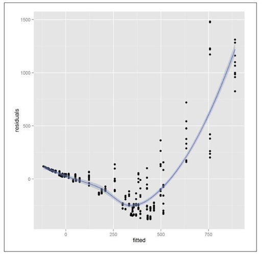
图15-3:基于ggplot2的残差与拟合值的诊断图
使用模型的真正妙处在于,你可基于任何一种你感兴趣的模型输入来预测结果。更有趣的是,如果模型中有一个时间变量,你就可预测未来。在本例中,让我们来看一看特定人群的感染率。出于对自己所属人群情况的好奇,我想知道30~34岁的非西班牙裔白人的感染率:
new_data <- data.frame(Age.Group = "30 to 34",Ethnicity = "Non-Hispanic Whites")predict(model4, new_data)## 1## 53.56
该模型预测的感染率为每10万人中会有54人。让我们把它与另一组的数据作对比:
subset( gonorrhoea, Age.Group == "30 to 34" & Ethnicity == "Non-Hispanic Whites" )## Year Age.Group Ethnicity Gender Rate## 7 2007 30 to 34 Non-Hispanic Whites Male 41.0## 19 2007 30 to 34 Non-Hispanic Whites Female 45.6## 127 2008 30 to 34 Non-Hispanic Whites Male 35.1## 139 2008 30 to 34 Non-Hispanic Whites Female 40.8## 247 2009 30 to 34 Non-Hispanic Whites Male 34.6## 259 2009 30 to 34 Non-Hispanic Whites Female 33.8## 367 2010 30 to 34 Non-Hispanic Whites Male 40.8## 379 2010 30 to 34 Non-Hispanic Whites Female 38.5## 487 2011 30 to 34 Non-Hispanic Whites Male 48.0## 499 2011 30 to 34 Non-Hispanic Whites Female 40.7
数据的范围为34~48 ,所以我们的预测稍微有点高。
