来自bit.ly的1.usa.gov数据
2011年,URL缩短服务bit.ly跟美国政府网站usa.gov合作,提供了一份从生成.gov或.mil短链接的用户那里收集来的匿名数据译注1。直到编写本书时为止,除实时数据译注2之外,还可以下载文本文件形式的每小时快照注1。
以每小时快照为例,文件中各行的格式为JSON(即JavaScript Object Notation,这是一种常用的Web数据格式)。例如,如果我们只读取某个文件中的第一行,那么你所看到的结果应该是下面这样:
- In [15]: path = 'ch02/usagov_bitly_data2012-03-16-1331923249.txt'
- In [16]: open(path).readline()
- Out[16]: '{ "a": "Mozilla\\/5.0 (Windows NT 6.1; WOW64) AppleWebKit\\/535.11 (KHTML, like Gecko) Chrome\\/17.0.963.78 Safari\\/535.11", "c": "US", "nk": 1, "tz": "America\\/New_York", "gr": "MA", "g": "A6qOVH", "h": "wfLQtf", "l": "orofrog", "al": "en-US,en;q=0.8", "hh": "1.usa.gov", "r": "http:\\/\\/www.facebook.com\\/l\\/7AQEFzjSi\\/1.usa.gov\\/wfLQtf", "u": "http:\\/\\/www.ncbi.nlm.nih.gov\\/pubmed\\/22415991", "t": 1331923247, "hc":1331822918, "cy": "Danvers", "ll": [ 42.576698, -70.954903 ] }\n'
Python有许多内置或第三方模块可以将JSON字符串转换成Python字典对象。这里,我将使用json模块及其loads函数逐行加载已经下载好的数据文件:
- import json
- path = 'ch02/usagov_bitly_data2012-03-16-1331923249.txt'
- records = [json.loads(line) for line in open(path)]
你可能之前没用过Python,解释一下上面最后那行表达式,它叫做列表推导式(list comprehension),这是一种在一组字符串(或一组别的对象)上执行一条相同操作(如json.loads)的简洁方式。在一个打开的文件句柄上进行迭代即可获得一个由行组成的序列。现在,records对象就成为一组Python字典了:
- In [18]: records[0]
- Out[18]:
- {u'a': u'Mozilla/5.0 (Windows NT 6.1; WOW64) AppleWebKit/535.11 (KHTML, like Gecko) Chrome/17.0.963.78 Safari/535.11', u'al': u'en-US,en;q=0.8',
- u'c': u'US',
- u'cy': u'Danvers',
- u'g': u'A6qOVH',
- u'gr': u'MA',
- u'h': u'wfLQtf',
- u'hc': 1331822918,
- u'hh': u'1.usa.gov',
- u'l': u'orofrog',
- u'll': [42.576698, -70.954903],
- u'nk': 1,
- u'r': u'http://www.facebook.com/l/7AQEFzjSi/1.usa.gov/wfLQtf',
- u't': 1331923247,
- u'tz': u'America/New_York',
- u'u': u'http://www.ncbi.nlm.nih.gov/pubmed/22415991'}
注意,Python的索引是从0开始的,不像其他某些语言是从1开始的(如R)。现在,只要以字符串的形式给出想要访问的键就可以得到当前记录中相应的值了:
- In [19]: records[0]['tz']
- Out[19]: u'America/New_York'
单引号前面的u表示unicode(一种标准的字符串编码格式)。注意,IPython在这里给出的是时区的字符串对象形式,而不是其打印形式:
- In [20]: print records[0]['tz']
- America/New_York
用纯Python代码对时区进行计数
假设我们想要知道该数据集中最常出现的是哪个时区(即tz字段),得到答案的办法有很多。首先,我们用列表推导式取出一组时区:
- In [25]: time_zones = [rec['tz'] for rec in records]
- In [25]: time_zones = [rec['tz'] for rec in records]
KeyError Traceback (most recent call last) /home/wesm/book_scripts/whetting/<ipython> in <module>() ——> 1 time_zones = [rec['tz'] for rec in records]
KeyError: 'tz'
晕!原来并不是所有记录都有时区字段。这个好办,只需在列表推导式末尾加上一个if 'tz'in rec判断即可:
- In [26]: time_zones = [rec['tz'] for rec in records if 'tz' in rec]
- In [27]: time_zones[:10]
- Out[27]:
- [u'America/New_York',
- u'America/Denver',
- u'America/New_York',
- u'America/Sao_Paulo',
- u'America/New_York',
- u'America/New_York',
- u'Europe/Warsaw',
- u'',
- u'',
- u'']
只看前10个时区,我们发现有些是未知的(即空的)。虽然可以将它们过滤掉,但现在暂时先留着。接下来,为了对时区进行计数,这里介绍两个办法:一个较难(只使用标准Python库),另一个较简单(使用pandas)。计数的办法之一是在遍历时区的过程中将计数值保存在字典中:
- def get_counts(sequence):
- counts = {}
- for x in sequence:
- if x in counts:
- counts[x] += 1
- else:
- counts[x] = 1
- return counts
如果非常了解Python标准库,那么你可能会将代码写得更简洁一些:
- from collections import defaultdict
- def get_counts2(sequence):
- counts = defaultdict(int) # 所有的值均会被初始化为0
- for x in sequence:
- counts[x] += 1
- return counts
我将代码写到函数中是为了获得更高的可重用性。要用它对时区进行处理,只需将time_zones传入即可:
- In [31]: counts = get_counts(time_zones)
- In [32]: counts['America/New_York']
- Out[32]: 1251
- In [33]: len(time_zones)
- Out[33]: 3440
如果想要得到前10位的时区及其计数值,我们需要用到一些有关字典的处理技巧:
- def top_counts(count_dict, n=10):
- value_key_pairs = [(count, tz) for tz, count in count_dict.items()]
- value_key_pairs.sort()
- return value_key_pairs[-n:]
现在我们就可以:
- In [35]: top_counts(counts)
- Out[35]:
- [(33, u'America/Sao_Paulo'),
- (35, u'Europe/Madrid'),
- (36, u'Pacific/Honolulu'),
- (37, u'Asia/Tokyo'),
- (74, u'Europe/London'),
- (191, u'America/Denver'),
- (382, u'America/Los_Angeles'),
- (400, u'America/Chicago'),
- (521, u''),
- (1251, u'America/New_York')]
你可以在Python标准库中找到collections.Counter类,它能使这个任务变得更简单:
- In [49]: from collections import Counter
- In [50]: counts = Counter(time_zones)
- In [51]: counts.most_common(10)
- Out[51]:
- [(u'America/New_York', 1251),
- (u'', 521),
- (u'America/Chicago', 400),
- (u'America/Los_Angeles', 382),
- (u'America/Denver', 191),
- (u'Europe/London', 74),
- (u'Asia/Tokyo', 37),
- (u'Pacific/Honolulu', 36),
- (u'Europe/Madrid', 35),
- (u'America/Sao_Paulo', 33)]
用pandas对时区进行计数
DataFrame是pandas中最重要的数据结构,它用于将数据表示为一个表格。从一组原始记录中创建DataFrame是很简单的:
- In [289]: from pandas import DataFrame, Series
- In [290]: import pandas as pd; import numpy as np
- In [291]: frame = DataFrame(records)
- In [292]: frame
- Out[292]:
- <class 'pandas.core.frame.DataFrame'>
- Int64Index: 3560 entries, 0 to 3559
- Data columns:
- _heartbeat_ 120 non-null values
- a 3440 non-null values
- al 3094 non-null values
- c 2919 non-null values
- cy 2919 non-null values
- g 3440 non-null values
- gr 2919 non-null values
- h 3440 non-null values
- hc 3440 non-null values
- hh 3440 non-null values
- kw 93 non-null values
- l 3440 non-null values
- ll 2919 non-null values
- nk 3440 non-null values
- r 3440 non-null values
- t 3440 non-null values
- tz 3440 non-null values
- u 3440 non-null values
- dtypes: float64(4), object(14)
- In [293]: frame['tz'][:10]
- Out[293]:
- 0 America/New_York
- 1 America/Denver
- 2 America/New_York
- 3 America/Sao_Paulo
- 4 America/New_York
- 5 America/New_York
- 6 Europe/Warsaw
- 7
- 8
- 9
- Name: tz
这里frame的输出形式是摘要视图(summary view),主要用于较大的DataFrame对象。frame['tz']所返回的Series对象有一个value_counts方法,该方法可以让我们得到所需的信息:
- In [294]: tz_counts = frame['tz'].value_counts()
- In [295]: tz_counts[:10]
- Out[295]:
- America/New_York 1251
- 521
- America/Chicago 400
- America/Los_Angeles 382
- America/Denver 191
- Europe/London 74
- Asia/Tokyo 37
- Pacific/Honolulu 36
- Europe/Madrid 35
- America/Sao_Paulo 33
然后,我们想利用绘图库(即matplotlib)为这段数据生成一张图片。为此,我们先给记录中未知或缺失的时区填上一个替代值。fillna函数可以替换缺失值(NA),而未知值(空字符串)则可以通过布尔型数组索引加以替换:
- In [296]: clean_tz = frame['tz'].fillna('Missing')
- In [297]: clean_tz[clean_tz == ''] = 'Unknown'
- In [298]: tz_counts = clean_tz.value_counts()
- In [299]: tz_counts[:10]
- Out[299]:
- America/New_York 1251
- Unknown 521
- America/Chicago 400
- America/Los_Angeles 382
- America/Denver 191
- Missing 120
- Europe/London 74
- Asia/Tokyo 37
- Pacific/Honolulu 36
- Europe/Madrid 35
利用counts译注3对象的plot方法即可得到一张水平条形图译注4:
- In [301]: tz_counts[:10].plot(kind='barh', rot=0)
最终结果如图2-1所示。我们还可以对这种数据进行很多处理。比如说,a字段含有执行URL短缩操作的浏览器、设备、应用程序的相关信息:
- In [302]: frame['a'][1]
- Out[302]: u'GoogleMaps/RochesterNY'
- In [303]: frame['a'][50]
- Out[303]: u'Mozilla/5.0 (Windows NT 5.1; rv:10.0.2) Gecko/20100101 Firefox/10.0.2'
- In [304]: frame['a'][51]
- Out[304]: u'Mozilla/5.0 (Linux; U; Android 2.2.2; en-us; LG-P925/V10e Build/FRG83G) AppleWebKit/533.1 (KHTML, like Gecko) Version/4.0 Mobile Safari/533.1'
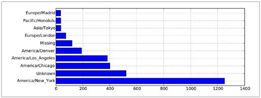
图2-1:1.usa.gov示例数据中最常出现的时区
将这些"agent"字符串译注5中的所有信息都解析出来是一件挺郁闷的工作。不过只要你掌握了Python内置的字符串函数和正则表达式,事情就好办了。比如说,我们可以将这种字符串的第一节(与浏览器大致对应)分离出来并得到另外一份用户行为摘要:
- In [305]: results = Series([x.split()[0] for x in frame.a.dropna()])
- In [306]: results[:5]
- Out[306]:
- 0 Mozilla/5.0
- 1 GoogleMaps/RochesterNY
- 2 Mozilla/4.0
- 3 Mozilla/5.0
- 4 Mozilla/5.0
- In [307]: results.value_counts()[:8]
- Out[307]:
- Mozilla/5.0 2594
- Mozilla/4.0 601
- GoogleMaps/RochesterNY 121
- Opera/9.80 34
- TEST_INTERNET_AGENT 24
- GoogleProducer 21
- Mozilla/6.0 5
- BlackBerry8520/5.0.0.681 4
现在,假设你想按Windows和非Windows用户对时区统计信息进行分解。为了简单起见,我们假定只要agent字符串中含有"Windows"就认为该用户为Windows用户。由于有的agent缺失,所以首先将它们从数据中移除:
- In [308]: cframe = frame[frame.a.notnull()]
其次根据a值计算出各行是否是Windows:
- In [309]: operating_system = np.where(cframe['a'].str.contains('Windows'),
- ...: 'Windows', 'Not Windows')
- In [310]: operating_system[:5]
- Out[310]:
- 0 Windows
- 1 Not Windows
- 2 Windows
- 3 Not Windows
- 4 Windows
- Name: a
接下来就可以根据时区和新得到的操作系统列表对数据进行分组了:
- In [311]: by_tz_os = cframe.groupby(['tz', operating_system])
然后通过size对分组结果进行计数(类似于上面的value_counts函数),并利用unstack对计数结果进行重塑:
- In [312]: agg_counts = by_tz_os.size().unstack().fillna(0)
- In [313]: agg_counts[:10]
- Out[313]:
- a Not Windows Windows
- tz
- 245 276
- Africa/Cairo 0 3
- Africa/Casablanca 0 1
- Africa/Ceuta 0 2
- Africa/Johannesburg 0 1
- Africa/Lusaka 0 1
- America/Anchorage 4 1
- America/Argentina/Buenos_Aires 1 0
- America/Argentina/Cordoba 0 1
- America/Argentina/Mendoza 0 1
最后,我们来选取最常出现的时区。为了达到这个目的,我根据agg_counts中的行数构造了一个间接索引数组:
- # 用于按升序排列
- In [314]: indexer = agg_counts.sum(1).argsort()
- In [315]: indexer[:10]
- Out[315]:
- tz
- 24
- Africa/Cairo 20
- Africa/Casablanca 21
- Africa/Ceuta 92
- Africa/Johannesburg 87
- Africa/Lusaka 53
- America/Anchorage 54
- America/Argentina/Buenos_Aires 57
- America/Argentina/Cordoba 26
- America/Argentina/Mendoza 55
然后我通过take按照这个顺序截取了最后10行:
- In [316]: count_subset = agg_counts.take(indexer)[-10:]
- In [317]: count_subset
- Out[317]:
- a Not Windows Windows
- tz
- America/Sao_Paulo 13 20
- Europe/Madrid 16 19
- Pacific/Honolulu 0 36
- Asia/Tokyo 2 35
- Europe/London 43 31
- America/Denver 132 59
- America/Los_Angeles 130 252
- America/Chicago 115 285
- 245 276
- America/New_York 339 912
这里也可以生成一张条形图。我将使用stacked=True来生成一张堆积条形图(如图2-2所示):
- In [319]: count_subset.plot(kind='barh', stacked=True)
由于在这张图中不太容易看清楚较小分组中Windows用户的相对比例,因此我们可以将各行规范化为“总计为1”并重新绘图(如图2-3所示):
- In [321]: normed_subset = count_subset.div(count_subset.sum(1), axis=0)
- In [322]: normed_subset.plot(kind='barh', stacked=True)
这里所用到的所有方法都会在本书后续的章节中详细讲解。
译注1:由于可以通过短链接伪造.gov后缀的URL,导致用户访问恶意域名,所以美国政府开始着手处理这种事情了。
译注2:以Feed形式提供。
注1:网址:http://www.usa.gov/About/developer-resources/1usagov.shtml。
译注3:应该是tz_counts 。
译注4:注意,一定要以pylab模式打开,否则这条代码没效果。包括很多缩写,pylab都直接弄好了,如果不是用这种模式打开,后面很多代码一样会遇到问题,虽然不是什么大毛病,但毕竟麻烦。后面如果遇到这没定义那找不到的情况,就请注意是不是因为这个。
译注5:即浏览器的USER_AGENT信息。
